[Paper Review - NLP] Mikolov et al., 2013 (CBOW & Skip Gram)

 

Efficient estimation of word representations in vector space (Mikolov et al., 2013)

Introduction

Traditional n-gram model

• Principle: prediction of next word based on previous n-1 words; probability of a sentence obtained by multiplying the probability (the n-gram model) of each word

  e.g., "This is a puppy"

  n = 1 (unigram): [This] [is] [a] [puppy] (this, is, a puppy)

  n = 2 (bigram): [This is] [is a] [a sentence] (this is, is a, a sentence)

  n = 3 (trigram): [This is a] [is a sentence] (this is a, is a sentence)

• Limits:

  i. insufficient amount of in-domain data (for ASR)

  ii. curse of dimensionality

  iii. difficulty of generalization (because the n-gram model has discrete space)

  iv. poor performance on word similarity tasks

Distributed representations of words as (continuous) vectors (vs. one-hot encoding)

e.g., queen → | 0.313 | 0.123 | 0.326 | 0.128 | 0.610 | 0.415 | 0.120 |

learning cost(?): the vocabulary size V * the number of parameters m (here 7)

• Previous work on representation of words as continuous vectors: Feedforward NNLM
• Motivation and goal: necessity of training more complex models on much larger data set with a modest dimensionality of the word vectors between 50-100; building a model that shows better performance on word similarity tasks (multiple degrees of similarity)

Model architectures

Some terms

• Computational complexity of a model: the number of parameters needed to fully train the model

• Training complexity is proportional to

  💡 O = E (number of training epochs; usually 3-50) * T (number of words in the training set; up to 1 billion) * Q (defined depending on model architecture)

Non-linear NN models

• Feedforward NNLM

  i. components: input, projection, hidden, and output layers

  ii. learning joint probability distribution of word sequences with word feature vectors using feedforward NN

  iii. input, output, and evaluation

  input: a concatenated feature vector of words

  output: the estimated probability of a sequence of n words

  a softmax function to evaluate the joint probability distribution of words

  iv. computational complexity per each training example

  💡 Q = N (1-of-V coded input) * D + N * D * H (hidden layer size) + H * V (vocabulary size)

The number of output layers can be reduced to log2|V| (base 2) using hierarchical softmax layers

• Recurrent NNLM: RNN-based NNLM

  i. components: input (the current word vector & hidden neuron values of the previous word), hidden, and output layers

  ii. predicting the current word

  iii. computational complexity per each training example

   💡 Q = H * H + H * V

  The number of output layers can be reduced to log_2|V| using hierarchical softmax layers.

  For more on hierarchical softmax:

  http://building-babylon.net/2017/08/01/hierarchical-softmax/

• 
  

• New log-linear models

  i. The main observation from the previous section was that most of the complexity is caused by the non-linear hidden layer in the model

  ii. While this is what makes NNs so attractive, a simpler model that might not be able to represent the data as precisely as NNs but can be trained on much more data efficiently

  iii. The two architectures

  
  
  
  
  
  
  

  
  

  
  

  
  

  
  

  
  

  
  

  
  

  
  

  Continuous Bag-of-words Model

  Similar to feedforward NNLM without the hidden layer

  Q = N * D + D * log_2(V)

  Continuous Skip-gram Model

  to predict words adjacent to the current word

  Q = C (max distance of the words) * (D + D * log_2(V))

  if C = 5, a number R in range < 1;C > is selected randomly, and then R words from past and those from future of the current word as correct labels. So, R * 2 word classifications with the current word as input and each of the R + R words as output.

Results

        Task description

            i. a comprehensive test set that contains 5 types of semantic questions and 9 types of

            syntactic questions (overall, 8869 semantic and 10675 syntactic questions)

• ii. evaluation: accuracy for each question type separately

  Maximization of accuracy

  Data: a Google News corpus for training the word vectors (6B tokens)

  i. restricted the vocabulary size to 1 million most frequent words

• ii. first evaluated models trained on subsets of the training data (the most frequent 30k words)

  
  
  
  

  
  

  
  

  
  

  
  

  iii. 3 training epochs with SGD and backpropagation; learning rate decreases from 0.025

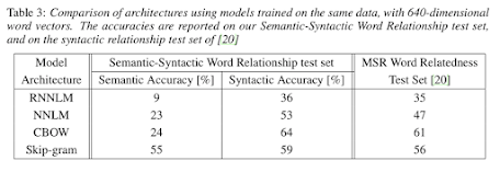
  Comparison of model architectures

  Data: several LDC corpora (320M words, 82k vocabulary)

• 
  
  
  
  
  
  
  

  
  

  
  

  
  

  
  

  
  

  
  

  
  

  
  

  
  

  
  

  
  

  
  

  
  

  
  

  Large scale parallel training of model 

  Several models trained on the Google News 6B data set, with mini-batch asynchronous gradient descent and the adaptive learning rate procedure (Adagrad)

Examples of the learned relationships

Conclusion

It is possible to train high quality word vectors using very simple model architectures

It is possible to compute very accurate high dimensional word vectors from a much larger data set

The word vectors can be successfully applied to automatic extension of facts in Knowledge Bases, and also for verification of correctness of existing facts